SIFT and RANSAC

The Homography matrix is a useful tool for remote measurements, perspective correction, image stitching, calculation of depth, and camera pose estimation. In my previous blog, I have discussed Template Matching, which is instrumental for object recognition and tracking and can automatically detect points required in solving the Homography matrix based on a reference image. However, Template Matching's limitations, scale, rotational, and intensity variant may not work effectively for images taken from a different orientation and distance. This blog will discuss a high-level definition of SIFT and RANSAC algorithm to solve Template Matching's limitations.

SIFT

Scale Invariant Feature Transform, known as SIFT, is a transformation algorithm invariant to image scale and rotation. Unlike in the Homography matrix and Template Matching, we do not need to describe what features we are looking for explicitly. The SIFT algorithm automatically does it for you.

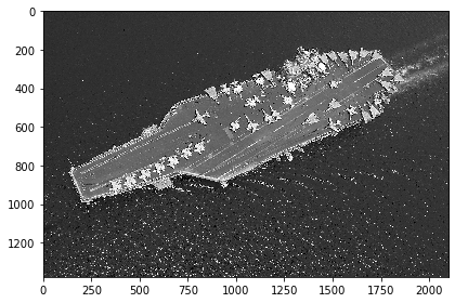
Fig 1. SIFT features

But how does SIFT work? SIFT involves a five-step process to identify potential key points in an image.

1. Scale-space peak selection

2. Key point Localization

3. Orientation Assignment

4. Key point descriptor

5. Key point matching.

Scale-space peak selection

To address the scale invariance limitation of Template Matching. Scale-space peak selection involves the following steps:

1. SIFT applies a consecutive convolution of Gaussian kernels across different source images' sizes to blur the image. The different sizes of the image are called octaves.

2. The difference of Gaussian (DOG) is then applied to various blurred images to find interesting key points in the picture.

3. Compare each pixel across its neighbors. We are trying to find the maximum intensity (local maxima of DOG) across different scales to determine the key points most apparent in terms of their neighbors.

Fig 2. Different octaves with different Gaussian Blur variance

Key point Localization

Scale-space peak location will return a lot of points in our image. However, not all points returned by the scale-space peak location are important. Key point location is used to remove non-feature key points using the Edge features (Hessian Matrix) and Low Contrast features (DOG). We want to remove the edges of the objects since most edges of different objects often look the same. Therefore, we need to compute for the corners instead of using the Hessian matrix. We also want to remove low-contrast features since they are barely visible in the image. From the figure below, we can see the result of an image after the key point localization.

Fig 3. Key point localization result (top image - before, bottom image - after)

Orientation Assignment

Essentially by this point, we have solved scale invariance. Now, Orientation Assignment solves another limitation of Template Matching, being rotation or orientation invariance. Determining the orientation of an object in our image can be difficult for machines. For example, humans can easily know that the object shown in the figure below is pointing upwards, but does our machine knows it is pointing upwards? How would you say that this object is different from objects with the same shape but pointing downwards?

Fig 4. Orientation object example

The SIFT algorithm takes the difference between the neighboring pixels and then looks at the angles and normalizes those angles towards the most significant difference. This step involves computing the gradients' magnitude and orientation and the image, then taking all the histograms of all the gradients. The peak is identified as the orientation of the pixel. There are two key points in orientation, 20 to 29 degrees and 300 to 309 degrees, shown in the figure below.

Fig 6. Histogram of Oriented Gradients

Keypoint Descriptor

The next step in SIFT algorithm is to look for features that would differentiate it among The next step in SIFT algorithm is to look for features that would differentiate it among others. We can describe these key points as a high dimensional vector, as shown in the figure below.

Fig 7. Key point high dimensional vector

In this step, we want to get the orientation of the key points surrounding pixels instead. We need to divide the neighboring pixels into a 16x16 window and then compute each pixel gradient. From those gradients, we get the 8-bin rotational histogram. Since we have eight values representing each 4x4 window's direction, each key point has a 128-dimensional vector. However, these vectors are Rotation and Illumination Dependent. To solve the rotation dependence, we need to subtract the key point's rotation from each orientation to compare several neighboring objects. Whereas in solving the illumination dependence, we solve it by looking at the thresholding values across our entire image.

Fig 8. Key point Descriptor result

Keypoint Matching

Given the Keypoint Descriptor results, we can now perform Keypoint matching as simple as looking at the nearest neighbor between images to match.

Fig 9. Key point Matching

Since a Homography matrix is sensitive to the source and destination points, one misclassified key point greatly affects the transformation. If all the key points are properly matched, how will we look for each source's four points and destination points in solving the Homography matrix? We need an algorithm to mathematically give us which points we need to consider to compute the transformation matrix.

RANSAC

Random Sample Consensus known as RANSAC is an iterative method for computing for the best Homography using random sampling. This method is used to find a set of points and fit a set of functions to these points to determine which points we need to consider. The RANSAC method takes random sample matches, computes a particular metric, and gets the matches' consensus to get the best fit.

Fig 10. RANSAC sample

First, the RANSAC method selects a pair of points and check if other points are in line with the selected pair shown in the figure below. The matching points in line with the selected pair are identified as points that head in the same direction. However, the case below presents zero inliers, which means there is no set of points with the same angle and transformation between the selected pair of points.

Fig 11. RANSAC counting inliers (Red line - Selected pair, White line - other points)

Now the RANSAC select another pair of points and check for the number of inliers. In the figure below, we can see that we now have four inliers.

Fig 12. RANSAC another set of inliers (Red line - Selected pair, White line - other points, Green line - inliers)

The RANSAC method do this process iteratively and monitor which pair has the highest number if inliers. After finding the pair with the most inliers, the method finds the average transformation/translation vector using only the inliers using least-squares fit.

Fig 13. RANSAC average translation vector

Extending the RANSAC method to the Homography matrix, we need to do the following:

1. Use SIFT to identify key points in our image.

2. Sample four different random points.

3. Compute for the Homography matrix of the four random points iteratively.

4. Get the Homography matrix with the highest number of inliers.

5. Compute the average Homography matrix among these inliers.
   

In computing for the Homography matrix, we need to manually define the source and destination points in the image, which can be a very tedious task. To automatically identify these points, we can implement the SIFT and RANSAC algorithms to successfully transform our images.